rRMSAnalyzer: package to analyze RiboMethSeq data

Abstract

RiboMethSeq is an innovative RNAseq-based approach, which was developed in 2015 to analyze 2’O-ribose methylation (2’Ome) at all sites of ribosomal RNAs (rRNA) at once, in yeast (Birkedal et al. 2014). This approach was then transferred to human using the Illumina technology (Marchand et al. 2016; Erales et al. 2017; Marcel et al. 2021). Briefly, the presence of 2’Ome protects the phosphodiester bond located at the 3’ of the 2’Ome nucleotide from alkaline hydrolysis. Thus, the presence of 2’Ome at the given nucleotide n induces under-representation of RNA fragments starting at the nucleotide n+1 and an over-representation of RNA fragments ending at the nucleotide n-1, allowing the extrapolation of 2’Ome levels at the corresponding nucleotide position n (or C-score) varying from 0 to 1 (Birkedal et al. 2014).

The rRMSAnalyzer package can be used for any kind of RNA and with all organisms. This package provides a set of user-friendly functions to compute C-scores from RiboMethSeq read end counts as input, adjust batch effect with ComBat-Seq, visualize the data and provide a table with the annotated human rRNA sites and their C-scores. This package provides a set of user-friendly functions to (i) compute C-scores from RiboMethSeq read-end counts as input,(ii) perform quality control of the dataset, (iii) adjust batch effect with ComBat-Seq, and (iv) provide tools to visualize, analyze the data and provide a table with the annotated human rRNA sites and their C-scores (Paraqindes et al., 2023), (v) return automated QC and analytic reports. Raw data processing to obtain read-end counts from sequencing data can be performed using our Nextflow pipeline ribomethseq-nf, as already described (Marchand et al. 2016).

General information

Help, bug reports and suggestions

To report a bug or any suggestion to improve the package, please let us know by opening a new issue on: https://github.com/RibosomeCRCL/rRMSAnalyzer/issues

Acknowledgements

We would like to thank all our collaborators for their advice and suggestions.

Funding

This project has been funded by the French Cancer Institute (INCa, PLBIO 2019-138 MARACAS), the SIRIC Program (INCa-DGOS-Inserm_12563 LyRICAN) and Synergie Lyon Cancer Foundation.

Installation

The latest version of rRMSAnalyzer package can be installed from Github with :

devtools::install_github("RibosomeCRCL/rRMSAnalyzer")
library(rRMSAnalyzer)

Initial preparation of the dataset

RiboClass

RiboClass is the main class of the package that enables the storage of both the data matrices (read-end counts and C-scores) and the associated metadata. It is automatically created when calling load_ribodata() (see Loading data).

It is a list containing three main elements, as described below:

Data: a list of dataframe, containing for each sample the 5’ and/or 3’ read-end counts provided by the user, and the calculated C-score.
Metadata: a dataframe, containing all the information related to the samples that can be provided by the user.
rRNA_names: a dataframe, reporting the names of the rRNA used in Data.

Some major function parameters (such as the normalization method used for C-score computation) are also kept in the RiboClass object as a reminder.

Loading data

Data to provide

Read-end counts

To use this package, the user must provide at least one csv/tsv file with the 5’, 3’ or 5’/3’ read-end counts resulting from RiboMethSeq data per sample. The folder structure containing the csv files is not important, as long as either the directory and its sub-directories contain the necessary csv/tsv files.

The name of the rRNA on which the read end counting was performed.
The position’s number on the rRNA.
The value of the read-end counts at the position.

Here is an example :

rRNA	Position on rRNA	read end count
18S	123	3746
18S	124	345
18S	125	324
18S	126	789
18S	127	1234

Note 1: it is not necessary to provide a header in the count files, because column index can be used in the function load_ribodata(), using count_value(), count_rnaid() and count_pos() arguments.

Note 2: if no metadata is specified (metadata = NULL), rRMSAnalyzer will try to fetch any csv files in the folder specified in count_path and its subfolders.

Metadata

The expected metadata is either a dataframe already in the R environment or a csv/tsv file.

Two columns are mandatory for the metadata :

filename: name of the csv file on disk containing the read-end counts described above. Do not modify it unless the filename has changed on disk.
samplename: rename the samples that will be analyzed and displayed on the plots. This column can be modified, as long as the sample names are unique.

After these two mandatory columns, the user can provide as many columns as needed for the analysis.

Here is an example of metadata for 3 samples:

filename (mandatory)	samplename (mandatory)	condition (optional) \|
sample1.csv	sample 1	condition 1
sample2.csv	sample 2	condition 1
sample3.csv	sample 3	condition 2

sample1.csv

sample 1

condition 1

sample2.csv

sample 2

condition 1

sample3.csv

sample 3

condition 2

Note: if no metadata is provided in load_ribodata() (metadata = NULL), an empty metadata will be created with the “filename” and “samplename” columns pre-filled. The “samplename” column will be identical to “filename”, but can be modified by the user.

Here is an example of auto-generated metadata:

filename	samplename
sample1.csv	sample1.csv
sample2.csv	sample2.csv
sample3.csv	sample3.csv

How to load the data

To load both data and metadata, and store them in a RiboClass, the function load_ribodata() is used.

The following example displays a call to load_ribodata(), with all arguments shown :

path <- system.file("extdata", package="rRMSAnalyzer") #change for your path

ribo <- load_ribodata(
                      #data & metadata files path
                      count_path = file.path(path,"miniglioma/"),
                      metadata = file.path(path,"metadata.csv"),
                      # data & metadata files separator
                      count_sep = "\t",
                      metadata_sep = ",",
                      # count data arguments :
                      count_header = FALSE,
                      count_value = 3,
                      count_rnaid = 1,
                      count_pos = 2,
                      # Metadata arguments :
                      metadata_key = "filename",
                      metadata_id = "samplename",
                      # C-score arguments :
                      flanking = 6,
                      method = "median",
                      ncores = 1)
#> ✔ Your data has been successfully loaded!

rRNA names

Provided

rRNA names are automatically obtained from the data and stored in a generated dataframe inside the RiboClass. It contains two columns :

original_name: original name of each rRNA (e.g NR_023363.1).
current_name: current name of each rRNA, reflecting any user’s change with rename_rna() function (see [Rename RNA]).

This dataframe is used to keep track of the original name, which often includes the NCBI’s accession ID.

Here is an example:

original_name	current_name
NR_023363.1_5S	5S
NR_046235.3_5.8S	5.8S
NR_046235.3_18S	18S
NR_046235.3_28S	28S

Custom

The user must not modify this dataframe manually. To rename or remove rRNA, the user can use rename_rna() and remove_rna(). The dataframe will be updated accordingly.

C-score calculation

What is a C-score ?

The C-score is a metric, calculated from the RiboMethSeq sequencing data, used to evaluate the level of 2’O-ribose methylation (2’Ome) at a given position in the rRNA.

The C-score is calculated by normalizing the end read count with respect to the local environment at each genomic position and directly indicates the rRNA 2’Ome level. The C-score ranges from 0 (i.e., no rRNA molecules of the sample are 2’Ome at this specific site) to 1 (i.e., all rRNA molecules of the sample are 2’Ome at this specific site). A C-score with an intermediate value between 0 to 1 means that the sample contains a mixture of un-2’Ome and 2’Ome rRNA molecules.

To obtain a robust estimate of the 2’Ome level, different C-scores can be determined depending on the arguments used to compute the local coverage. In particular, the estimation method and the size of the local coverage to be considered can be changed.

By default, the local coverage is estimated by calculating the median of the 5’ read-end counts in a flanking region of 6 (i.e., 6 nucleotides downstream the nucleotide n and 6 upstream the nucleotide n, where n is the nucleotid directly following the 2’Ome site of interest). This package provides the ability to change these two arguments either when loading the data or during the analysis.

When using the load_ribodata() function, a C-score is automatically calculated for all genomic positions of the rRNA. The C-score is computed using either the default arguments of the load_ribodata() function or user-defined arguments as follows:

load_ribodata(count.path = "/path/to/csv/",
              metadata = "/path/to/metadata.csv",
              # everything below is linked to C-score computation
              flanking = 6, # flanking region size
              method = "median", # use mean or median on flanking region's values
              ncores = 8 # number of CPU cores to use for computation
              )

C-score computation during the analysis

During the analysis, the C-score calculating arguments (method and size of the flanking region) can be modified using the compute_cscore() function, which will automatically update the C-score in the RiboClass.

In the following example, both the flanking region’s size of the local coverage and the computation method have been modified:

# Compute the C-score using different arguments,
# including calculation of the local coverage using the mean instead of the median
ribo <- compute_cscore(ribo,
                       flanking = 4,
                       method = "mean")

Important: this function will override the previous C-score of the RiboClass.

Quality control

Due to technical limitations, it is sometimes necessary to conduct wet-lab preparations of large cohorts in several batches. The main risk when making several batches is to introduce technical biases or batch effect in the dataset.

Content of the QC report

A quality control (QC) report can be performed. It uses several metrics to help identify outlier samples and/or batch effects, including read-end counts and the C-score itself at all the 7217 genomic positions. The QC verifies that the coverage is uniform and reproducible between samples, eliminating the possibility of bias due to sequencing and outliers.

QC can be either performed using a panel of ready to use functions, which correspond to data visualization, or automatically.

The automatic QC report can be generated using the report_qc() function:

With the ribo_toy example, the column that contains the information about samples batches is called “run”. The name is thus given to the library_col argument but it can be also left empty.

report_qc(ribo = ribo_toy, library_col = "run")

The QC report includes the following visualizations:

Read-end counts distribution by sample (boxplot_count())
Relative log coverage (i.e., end read count) by sample (plot_rlc())
rRNA fraction of read-end counts per sample (plot_count_fraction())
Heatmap summarizing the correlation matrix of the read-end counts (heatmap_annotated())
Correspondence analysis of the read-end counts (plot_coa())
Principal component analysis (plot_pca())

Correlation matrix

To add outlier annotations on the heatmap, get_outliers() function must be used. This function computes all the outliers identified in the QC and returns a data frame summary for use in plot_heatmap_annotated()

Here is an example of correlation matrix with outlier identification:

qcdata <- rRMSAnalyzer::get_outliers(ribo)
plot_heatmap_annotated(ribo, qcdata)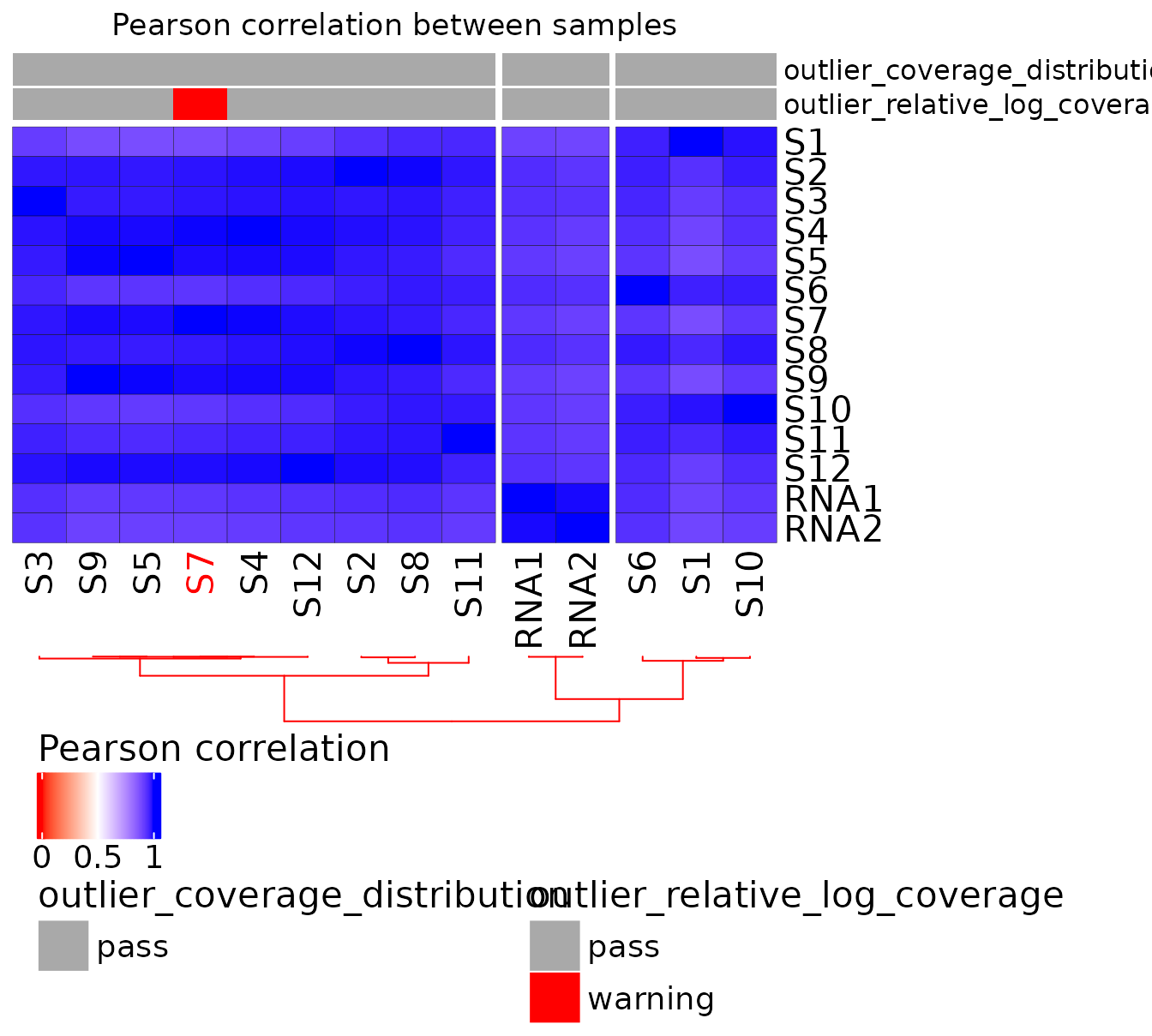

Output of the QC report

Information issued from the QC report can be return as followed:

Here is an example of QC output:

output_dir <- getwd()
# To display the output
knitr::kable(qcdata, "html") %>% kable_styling("striped") %>% scroll_box(width = "100%", height = "500px")

	samplename	condition	run	filename	median_coverage	coverage_quality	rlc_median	rlc_median_quality	total_outliers
S1	S1	cond1	L2	S1_5_counts.csv	1761	pass	0.0575140	pass	0
S2	S2	cond2	L1	S2_5_counts.csv	1292	pass	-0.3439012	pass	0
S3	S3	cond2	L2	S3_5_counts.csv	2212	pass	0.3954259	pass	0
S4	S4	cond2	L1	S4_5_counts.csv	2147	pass	0.3337012	pass	0
S5	S5	cond2	L2	S5_5_counts.csv	1682	pass	-0.0113976	pass	0
S6	S6	cond2	L2	S6_5_counts.csv	1774	pass	0.0499721	pass	0
S7	S7	cond2	L1	S7_5_counts.csv	696	pass	-1.2547609	warning	1
S8	S8	cond1	L1	S8_5_counts.csv	1759	pass	0.0618611	pass	0
S9	S9	cond1	L2	S9_5_counts.csv	1394	pass	-0.2504866	pass	0
S10	S10	cond1	L1	S10_5_counts.csv	1625	pass	-0.0767012	pass	0
S11	S11	cond1	L1	S11_5_counts.csv	1632	pass	-0.0471291	pass	0
S12	S12	cond1	L2	S12_5_counts.csv	1683	pass	0.0062753	pass	0
RNA1	RNA1	RNA ref	L1	RNA1_5_counts.csv	1593	pass	-0.1061994	pass	0
RNA2	RNA2	RNA ref	L2	RNA2_5_counts.csv	2316	pass	0.3822330	pass	0

# To save the output
write.table(qcdata,file.path(output_dir,"quality_control.csv"),sep="\t",row.names=FALSE,quote = FALSE)

Comments

A Comments section is available in the QC report to add some personal comments. To do so, a Rmarkdown file should be created and saved in the working directory. Then, path to this report should be given in the comments argument of the report_qc() function.

report_qc(ribo = ribo, specie = "human", library_col = "run", comments = "./path/to/comment_QC.Rmd")

Example of comments in rmd extension

```{=html} 
<style type="text/css">
  body {
    font-family: Helvetica;
  }

  /* Apply a skyblue background to the blocks <details> */
  details {
    background-color: #9ecae1;
    padding: 10px;
    border-radius: 5px;
  }
</style>
``` # erase this '#' and this sentence
<details>

<summary><b> ℹ Comments on the report  </b></summary>
<div markdown="1">
<p>
Text can be entered from here ...

Subtitle can be added with '##' symbol:

## 5.3 Level 2 title {-} #this symbol {-} avoid continue the numbering of the table of content

...to here. Those last 2 lines below must be kept. They are usefull for the layout.
</div>
</details>
  
#copy/past in an rmd file
#apply in the report_qc() function
#report_qc(ribo = ribo….)

Batch effect

Batch effect identification

Technical bias (i.e., batch effect) can be identified by plotting C-scores at all the genomic positions of the rRNA for each sample on a PCA (see also [Visualization with PCA] for more uses).

Since more than 1.5% of the C-score corresponds to non-biological noise, normalization during C-score calculation should limit the dispersion of the samples based on their C-score at all genomic positions in the whole series. Thus, Principal Component Analysis (PCA) on C-scores helps to identify putative batch effects that can be corrected using the inter-normalization option (ComBat-seq tool) (Zhang et al, 2020; Paraqindes et al, 2023).

The graph shows a Principal Component Analysis (PCA) plot illustrating the distance between each sample based on its C-score at all genomic positions. The samples are colored by library.

Here is an example:

# Plot a Principal Component Analysis (PCA) whose colors depend on the "run" column in metadata
plot_pca(ribo = ribo,
         color_col = "run")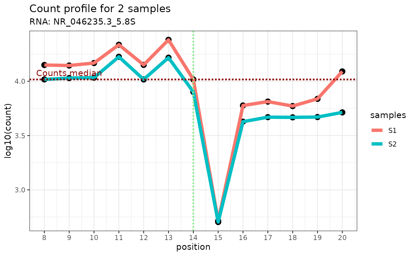

In this example, the technical replicates RNA1 and RNA2 included in library 1 and 2 respectively, are distant from each other on the PC1 axis. Moreover, the samples should not be grouped by library or batch. The following section will resolve this batch effect.

Batch effect adjustment

Batch effect of RiboMethSeq data can be adjusted using the ComBat-seq method (Paraqindes et al, 2023 ; Zhang, et al, 2020). The rRMSAnalyzer package includes a wrapper (adjust_bias) to perform ComBat-seq adjustment which provides a new RiboClass with adjusted read end count values and C-scores automatically recalculated with the same setup arguments.

data("ribo_toy")
# If necessary, adjust any technical biases using ComBat-Seq.
# Here, as an example, we use the "run" column in metadata.
ribo_adjusted <- adjust_bias(ribo_toy, batch = "run")
#> Found 2 batches
#> Using null model in ComBat-seq.
#> Adjusting for 0 covariate(s) or covariate level(s)
#> Estimating dispersions
#> Fitting the GLM model
#> Shrinkage off - using GLM estimates for parameters
#> Adjusting the data
#> Recomputing c-score with the following parameters :
#> - C-score method : median
#> - Flanking window : 6

Batch effect adjustment can be verified using the plot_pca function on the new RiboClass:

plot_pca(ribo_adjusted,"run")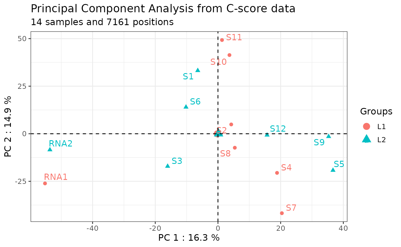

After batch effect adjustment using ComBat-seq method, the two technical replicates RNA1 and RNA2 show reduced dispersion, and the samples are separated on the PCA axes independently of the library they belong to.

Verifying local coverage

The C-score depends on the local coverage around the site. For a simple visualization of the read end count coverage of the flanking region of a given genomic position of interest, use the plot_counts_env() function. Two plotting methods are available:

display all samples (default arguments): by displaying the end read count coverage of all samples using a boxplot at the +/-6 genomic position relative to the genomic position of interest (green box). A pink box is displayed if there is other modification in the window. Such a plot is automatically used when samples = “all”. The median of the read end count and coverage limit are shown as two dashed red lines.

Here is an example:

plot_counts_env(ribo_adjusted,"NR_046235.3_5.8S",14)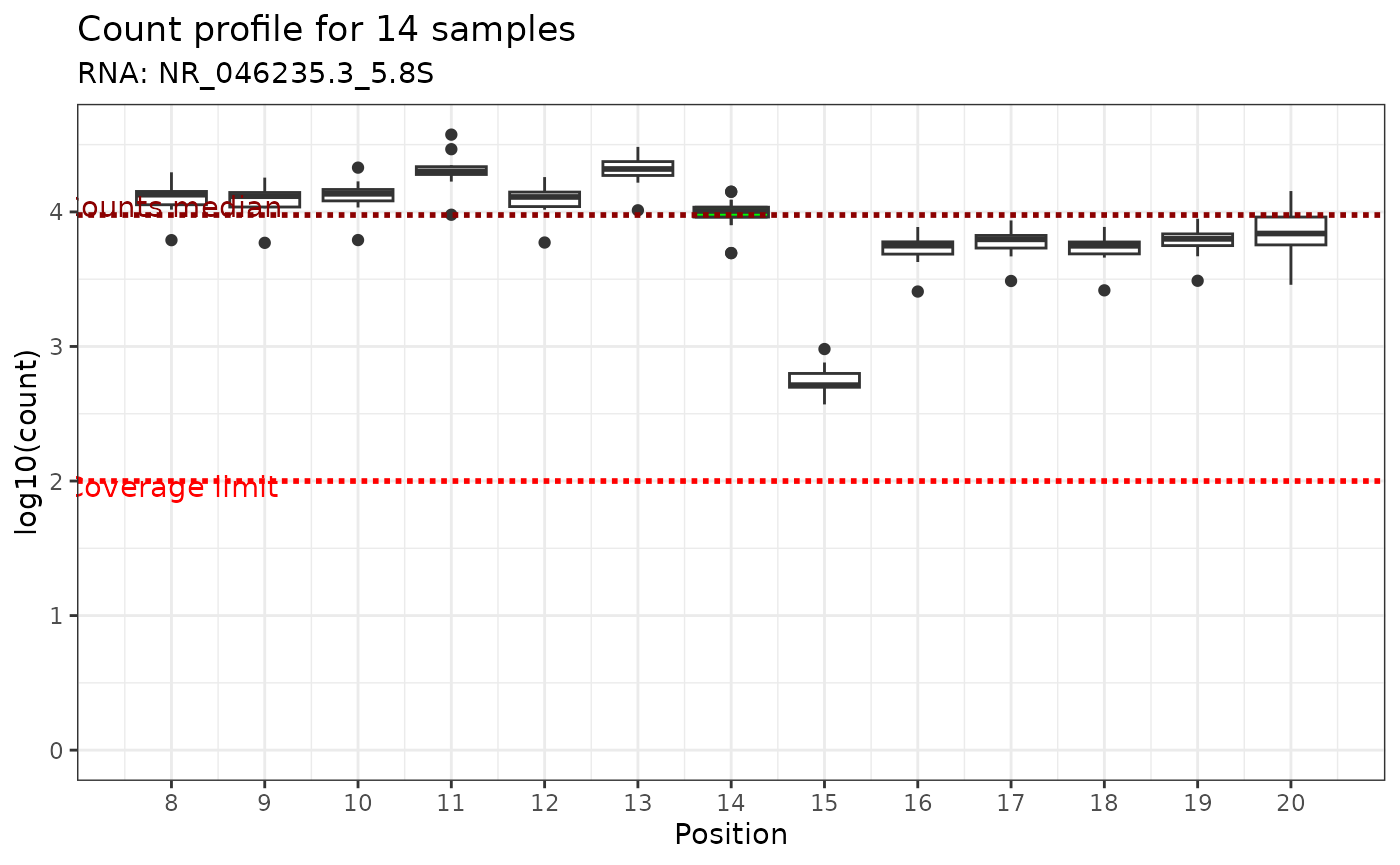

sample of interest: by displaying the end read count coverage of the sample of interest only using the profile at the +/-6 genomic position relative to the genomic position of interest (vertical green line). The median of the read end count is displayed as a horizontal dotted red line.

Here is an example:

plot_counts_env(ribo_adjusted,"NR_046235.3_5.8S",14,c("S1","S2"))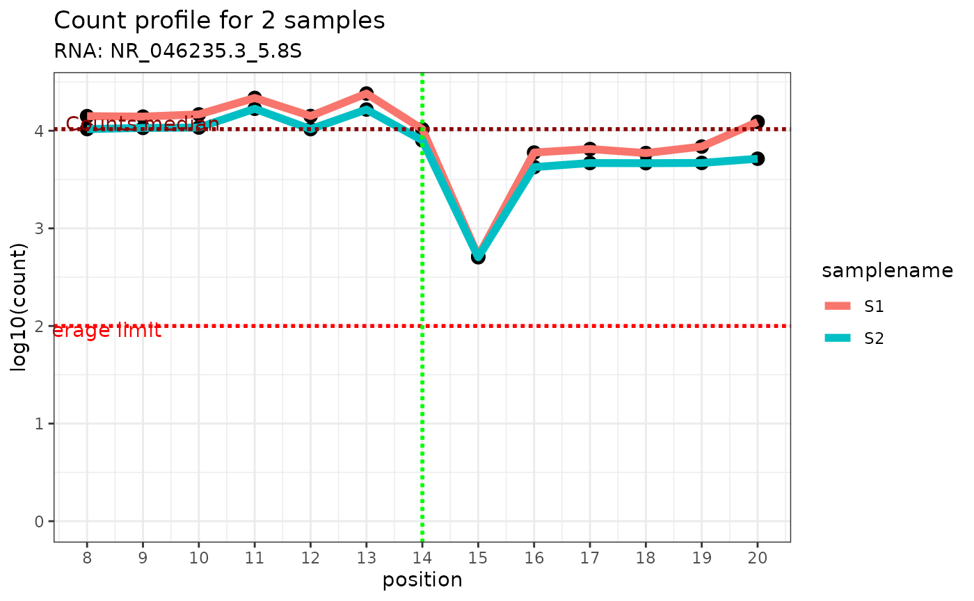

Data formatting for subsequent analyses

Sample manipulation

Keep or remove samples

A sample subset can be easily analyzed by specifying which samples to keep or which to remove. The user can then create a new RiboClass object containing the data and metadata of the samples of interest. In both cases, only the metadata of the remaining samples are kept in the RiboClass object, so no manual updating is required.

Here is an example of how to create a new RiboClass by retaining two samples of interest (“S1” and “S2”):

ribo_2samples <- keep_ribo_samples(ribo_adjusted,c("S1","S2"))
print(ribo_2samples)
#> a RiboClass with 2 samples and 4 RNA(s) :
#> Name : NR_023363.1_5S, length : 121
#>  Name : NR_046235.3_5.8S, length : 157
#>  Name : NR_046235.3_18S, length : 1869
#>  Name : NR_046235.3_28S, length : 5070

Here is an example to generate a new RiboClass by removing two samples (“RNA1” and “RNA2”):

ribo_adjusted <- remove_ribo_samples(ribo_adjusted,c("RNA1","RNA2"))
print(ribo_adjusted)
#> a RiboClass with 12 samples and 4 RNA(s) :
#> Name : NR_023363.1_5S, length : 121
#>  Name : NR_046235.3_5.8S, length : 157
#>  Name : NR_046235.3_18S, length : 1869
#>  Name : NR_046235.3_28S, length : 5070

In both cases, only the remaining samples’ metadata are kept in the RiboClass object. There is no need to update it manually.

rRNA manipulation and annotation

rRNA manipulation

Remove rRNA

A subset of rRNA can be easily analyzed by specifying the rRNA to be removed. The user can thus create a new RiboClass object containing the data of the rRNAs of interest, without affecting the metadata of the samples.

Here is an example where the rRNA 5S is removed:

ribo_adjusted <- remove_rna(ribo, rna_to_remove = "NR_023363.1_5S")
print(ribo_adjusted)
#> a RiboClass with 14 samples and 3 RNA(s) :
#> Name : NR_046235.3_5.8S, length : 157
#>  Name : NR_046235.3_18S, length : 1869
#>  Name : NR_046235.3_28S, length : 5070

Rename rRNA

The annotation of rRNA 2’Ome sites using the lists provided by this package requires the use of specific rRNA names.

Here is an example to check if the rRNA names provided by the user in the RiboClass match the ones used by this package :

data("human_methylated")
cat("human_methylated's rna names: ", unique(human_methylated$rRNA),"\n")
#> human_methylated's rna names:  5.8S 18S 28S
cat("ribo's rna names: ", as.character(ribo_adjusted$rna_names$current_name))
#> ribo's rna names:  NR_046235.3_5.8S NR_046235.3_18S NR_046235.3_28S

In this example, the names are different and need to be updated before annotation.

The rename_rna() function automatically updates the rRNA names given by the rRNA size order:

ribo_adjusted <- rename_rna(ribo_adjusted,
                            new_names = c("5.8S", "18S", "28S")) 
                            # from the shortest rRNA in our RiboClass to the longest.

Annotation of rRNA 2’Ome sites

The rRMSAnalyzer package calculates a C-score for each genomic position of the rRNAs. However, not every site of the reference 2’Ome rRNA is necessarily methylated. Therefore, it is expected that the user provides a list of potentially methylated sites of interest, called “annotated sites”. This will make it easier to restrict further analysis to this list of sites. By default, rRMSAnalyzer package includes its own human annotated sites.

Included annotation : Human 2’Ome rRNA sites

By default, rRMSAnalyzer package includes three dataframes containing the positions and the annotations of the human rRNA 2’Ome sites:

human_methylated: a dataframe, containing the 112 known 2’Ome sites for the human rRNAs.
human_suspected: a dataframe, containing the 17 sites that are putative 2’Ome sites for the human rRNAs, as described in the litterature.
human_both_methylated_and_suspected: a dataframe, containing the 129 sites of both known 2’Ome sites and sites that are putative 2’Ome sites for the human rRNAs.

Customize 2’Ome sites annotations

Instead of using the list of human rRNA 2’Ome sites provided by the rRMSAnalyzer package, the user can provide their own list of annotated sites which will be attached to the RiboClass object using the annotate_site() function (see Section : annotation of rRNA 2’Ome sites).

This annotate_site() function expects an “annot” argument which must be a dataframe object that contains the following three mandatory columns :

RNA name: the name of the rRNA, matching the rRNA name of the RiboClass.
Position on RNA: the number of the position on the rRNA.
Nomenclature: the name given to the site of interest.

You can see an example below :

Position	rRNA	Nomenclature
15	5.8S	Um14
76	5.8S	Gm75
28	18S	Am27

Annotate rRNA sites

The 2’Ome sites of interest must be attached to the RiboClass object for further analysis using the annotate_site() function with either the provided annotations or custom annotations (see Customize 2’Ome sites annotations).

Here is an example using the included human methylated annotations:

ribo_adjusted <- annotate_site(ribo_adjusted,
                               annot = human_methylated,
                               anno_rna = "rRNA",
                               anno_pos = "Position",
                               anno_value = "Nomenclature")

Note : rRMSAnalyzer will display a warning message when there is a mismatch between the annot and RiboClass rRNA names.

This vignette also provides some explanations on how to create your own sites annotation dataset with Customize 2’Ome sites annotations.

Analysis design for multiple comparisons

Although comparison of two groups can be computed using the analytic report functions (e.g., report_2ome_sites or report_diff_sites – (see [2’Ome profiling report] or 2’Ome site-by-site report)) thanks to the “condition” column of the metadata, this section needs to be considered to perform multiple comparisons (i.e., more than 2 groups). The following section Addition of new columns in the metadata is required for the two reports while the section Comparison table is required for report_diff_sites only.

Addition of new columns in the metadata

To perform multiple group comparison, the metadata needs to be implemented with additional information on the experimental conditions in order to create as much as novel Riboclass required to perform all the comparison. The metadata are stored in the RiboClass object once it has been created. To change the metadata, (i) amend the metadata csv.file used to create the RiboClass (see How to load the data) and (ii) recreate the RiboClass using the load_ribodata() function.

Here is an example:

VariableA (9 samples) has 1 control (ctrl) and 2 cases (P1 and P2) with 3 replicates for each (total = 9 samples).
VariableB (4 samples) has 1 control (ctrl) and 1 case (P2) with 2 replicates for each (total = 4 samples).
VariableC (6 samples) has 1 control (ctrl) and 1 case (P2) with 3 replicates for each (total = 6 samples).

(i) Update of the metadata .csv file

->>> Here is the initial metadata in the RiboClass:

filename	samplename	condition	treatment	lib
S26_R1.5_counts.csv	variableB_N2_P2	variableB	P2	L2
S27_R1.5_counts.csv	variableA_N2_P1	variableA	P1	L2
S28_R1.5_counts.csv	variableC_N1_ctrl	variableC	ctrl	L2
S30_R1.5_counts.csv	variableB_N1_P2	variableB	P2	L2
S31_R1.5_counts.csv	variableC_N2_P2	variableC	P2	L2
S32_R1.5_counts.csv	variableA_N3_P1	variableA	P1	L2
S33_R1.5_counts.csv	variableA_N3_ctrl	variableA	ctrl	L2
S34_R1.5_counts.csv	variableC_N3_ctrl	variableC	ctrl	L2
S35_R1.5_counts.csv	variableA_N1_P2	variableA	P2	L2
S36_R1.5_counts.csv	variableA_N2_ctrl	variableA	ctrl	L2
S37_R1.5_counts.csv	variableC_N2_ctrl	variableC	ctrl	L2
S38_R1.5_counts.csv	variableA_N2_P2	variableA	P2	L2
S39_R1.5_counts.csv	variableC_N1_P2	variableC	P2	L2
S40_R1.5_counts.csv	variableB_N1_ctrl	variableB	ctrl	L2
S41_R1.5_counts.csv	variableA_N1_P1	variableA	P1	L2
S42_R1.5_counts.csv	variableA_N1_ctrl	variableA	ctrl	L2
S43_R1.5_counts.csv	variableC_N3_P2	variableC	P2	L2
S44_R1.5_counts.csv	variableB_N2_ctrl	variableB	ctrl	L2
S45_R1.5_counts.csv	variableA_N3_P2	variableA	P2	L2

->>> A simple way to format the metadata is to add three columns, one for each experimental condition (i.e., termed “variable A to C” in this example) in which the second experimental condition is implemented (i.e., termed “ctrl, P1, P2” in this example).
Here is an example of the first design of the novel metadata:

filename	samplename	variableA	variableB	variableC	condition	treatment	lib
S26_R1.5_counts.csv	variableB_N2_P2	NA	P2	NA	variableB	P2	L2
S27_R1.5_counts.csv	variableA_N2_P1	P1	NA	NA	variableA	P1	L2
S28_R1.5_counts.csv	variableC_N1_ctrl	NA	NA	ctrl	variableC	ctrl	L2
S30_R1.5_counts.csv	variableB_N1_P2	NA	P2	NA	variableB	P2	L2
S31_R1.5_counts.csv	variableC_N2_P2	NA	NA	P2	variableC	P2	L2
S32_R1.5_counts.csv	variableA_N3_P1	P1	NA	NA	variableA	P1	L2
S33_R1.5_counts.csv	variableA_N3_ctrl	ctrl	NA	NA	variableA	ctrl	L2
S34_R1.5_counts.csv	variableC_N3_ctrl	NA	NA	ctrl	variableC	ctrl	L2
S35_R1.5_counts.csv	variableA_N1_P2	P2	NA	NA	variableA	P2	L2
S36_R1.5_counts.csv	variableA_N2_ctrl	ctrl	NA	NA	variableA	ctrl	L2
S37_R1.5_counts.csv	variableC_N1_ctrl	NA	NA	ctrl	variableC	ctrl	L2
S38_R1.5_counts.csv	variableA_N2_P2	P2	NA	NA	variableA	P2	L2
S39_R1.5_counts.csv	variableC_N2_P2	NA	NA	P2	variableC	P2	L2
S40_R1.5_counts.csv	variableB_N1_ctrl	NA	ctrl	NA	variableB	ctrl	L2
S41_R1.5_counts.csv	variableA_N1_P1	P1	NA	NA	variableA	P1	L2
S42_R1.5_counts.csv	variableA_N1_ctrl	ctrl	NA	NA	variableA	ctrl	L2
S43_R1.5_counts.csv	variableC_N3_P2	NA	NA	P2	variableC	P2	L2
S44_R1.5_counts.csv	variableB_N3_ctrl	NA	ctrl	NA	variableB	ctrl	L2
S45_R1.5_counts.csv	variableA_N3_P2	P2	NA	NA	variableA	P2	L2

->>> If the analysis includes comparison of 2 conditions independently of the other (e.g., all ctrl vs all P2), the addition of a single column is required (i.e., “comp1” in this example).
Here is an example of the second design of the novel metadata:

filename	samplename	comp1	condition	treatment	lib
S26_R1.5_counts.csv	variableB_N2_P2	P2	variableB	P2	L2
S27_R1.5_counts.csv	variableA_N2_P1	NA	variableA	P1	L2
S28_R1.5_counts.csv	variableC_N1_ctrl	ctrl	variableC	ctrl	L2
S30_R1.5_counts.csv	variableB_N1_P2	P2	variableB	P2	L2
S31_R1.5_counts.csv	variableC_N2_P2	P2	variableC	P2	L2
S32_R1.5_counts.csv	variableA_N3_P1	NA	variableA	P1	L2
S33_R1.5_counts.csv	variableA_N3_ctrl	ctrl	variableA	ctrl	L2
S34_R1.5_counts.csv	variableC_N3_ctrl	ctrl	variableC	ctrl	L2
S35_R1.5_counts.csv	variableA_N1_P2	P2	variableA	P2	L2
S36_R1.5_counts.csv	variableA_N2_ctrl	ctrl	variableA	ctrl	L2
S37_R1.5_counts.csv	variableC_N1_ctrl	ctrl	variableC	ctrl	L2
S38_R1.5_counts.csv	variableA_N2_P2	P2	variableA	P2	L2
S39_R1.5_counts.csv	variableC_N2_P2	P2	variableC	P2	L2
S40_R1.5_counts.csv	variableB_N1_ctrl	ctrl	variableB	ctrl	L2
S41_R1.5_counts.csv	variableA_N1_P1	NA	variableA	P1	L2
S42_R1.5_counts.csv	variableA_N1_ctrl	ctrl	variableA	ctrl	L2
S43_R1.5_counts.csv	variableC_N3_P2	P2	variableC	P2	L2
S44_R1.5_counts.csv	variableB_N3_ctrl	ctrl	variableB	ctrl	L2
S45_R1.5_counts.csv	variableA_N3_P2	P2	variableA	P2	L2

->>> If the analysis includes comparison of a pool of 2 conditions independently of the other (e.g., all ctrl vs all P1+P2), the addition of a single column is required (i.e., “comp1” in this example) with a new annotation (i.e., “P” = P1 or P2).
Here is an example of the third design of the novel metadata:

filename	samplename	comp1	condition	treatment	lib
S26_R1.5_counts.csv	variableB_N2_P2	P	variableB	P2	L2
S27_R1.5_counts.csv	variableA_N2_P1	P	variableA	P1	L2
S28_R1.5_counts.csv	variableC_N1_ctrl	ctrl	variableC	ctrl	L2
S30_R1.5_counts.csv	variableB_N1_P2	P	variableB	P2	L2
S31_R1.5_counts.csv	variableC_N2_P2	P	variableC	P2	L2
S32_R1.5_counts.csv	variableA_N3_P1	P	variableA	P1	L2
S33_R1.5_counts.csv	variableA_N3_ctrl	ctrl	variableA	ctrl	L2
S34_R1.5_counts.csv	variableC_N3_ctrl	ctrl	variableC	ctrl	L2
S35_R1.5_counts.csv	variableA_N1_P2	P	variableA	P2	L2
S36_R1.5_counts.csv	variableA_N2_ctrl	ctrl	variableA	ctrl	L2
S37_R1.5_counts.csv	variableC_N1_ctrl	ctrl	variableC	ctrl	L2
S38_R1.5_counts.csv	variableA_N2_P2	P	variableA	P2	L2
S39_R1.5_counts.csv	variableC_N2_P2	P	variableC	P2	L2
S40_R1.5_counts.csv	variableB_N1_ctrl	ctrl	variableB	ctrl	L2
S41_R1.5_counts.csv	variableA_N1_P1	P	variableA	P1	L2
S42_R1.5_counts.csv	variableA_N1_ctrl	ctrl	variableA	ctrl	L2
S43_R1.5_counts.csv	variableC_N3_P2	P	variableC	P2	L2
S44_R1.5_counts.csv	variableB_N3_ctrl	ctrl	variableB	ctrl	L2
S45_R1.5_counts.csv	variableA_N3_P2	P	variableA	P2	L2

(ii) create a new Riboclass:

ribo_exp_design <- load_ribodata(count_path = ..., metadata = "./new_metadata.csv")

Comparison table

To perform an automated multiple group comparison using the report_diff_sites function, a dataframe containing all the biological comparisons should be prepared. This dataframe is created using the code provided below and including in a new RiboClass created using the load_ribodata() function and the argument comparison.

Here is an example:

The study includes 3 experimental conditions termed “variable A to C” (e.g., wild-type, mutation 1, mutation 2) that has been exposed to another condition termed “ctrl, P1 and P2 (e.g., untreated vs treatment with 2 different concentrations). All these experimental conditions have been performed in replicates termed “N”. In summary, it includes:
- VariableA has 1 control (ctrl) and 2 cases (P1 and P2) with 3 replicates each (total = 9 samples)
- VariableB has 1 control (ctrl) and 1 case (P2) with 2 replicates each (total = 4 samples)
- VariableC has 1 control (ctrl) and 1 case (P2) with 3 replicates or each (total = 6 samples)

The objectives are to perform 2 comparisons in the “variableA” condition only, as summarized here:

comp (mandatory)	ctrl (mandatory)	cases (mandatory)
comp1 (mandatory)	ctrl	P1
comp2 (optional)	ctrl	P2

comp1 (mandatory)

ctrl

comp2 (optional)

ctrl

(i) Creation of the dataframe for the report_diff_sites function:

Here is the code to create the comparison table

#---------------------Creation of the comparison table--------------------------
# Here is the comparison table needed for this example data
comparisons <- tibble::tibble(
  comp = c("comp1", "comp2"),
  ctrl = c("ctrl", "ctrl"),
  cases = c("P1", "P2")
)

(ii) Creation of a new RiboClass including only the required samples

Here is an example to extract a new RiboClass incuding only the samples required to perfom the multiple comparison. It refers to the metadata/RiboClass created in the previous section “(i) Update of the metadata .csv file”, in the subsection “If the analysis includes comparison of 2 conditions independently of the other”.

Store the subset samples required for the analysis using the column names of the metadata created in the previous section “Addition of new columns in the metadata”

kept_samples <- ribo_adj_annot$metadata %>% #use the new RiboClass created in the previous section “Addition of new columns in the metadata”  
  dplyr::filter(!is.na(variableA)) %>% # filter the lines in the metadata to keep only those that are not NA in the "variableA" column
  dplyr::pull(samplename)

# create a copy of the RiboClass with the subset of samples
ribo_adj_annot_variableA <- keep_ribo_samples(ribo_adj_annot,kept_samples) # save the new RiboClass including only the samples with information in the “variableA” column

filename	samplename	variableA	treatment	condition	lib
S27_R1.5_counts.csv	variableA_N2_P1	P1	variableA	P1	L2
S32_R1.5_counts.csv	variableA_N3_P1	P1	variableA	P1	L2
S33_R1.5_counts.csv	variableA_N3_ctrl	ctrl	variableA	ctrl	L2
S35_R1.5_counts.csv	variableA_N1_P2	P2	variableA	P2	L2
S36_R1.5_counts.csv	variableA_N2_ctrl	ctrl	variableA	ctrl	L2
S38_R1.5_counts.csv	variableA_N2_P2	P2	variableA	P2	L2
S41_R1.5_counts.csv	variableA_N1_P1	P1	variableA	P1	L2
S42_R1.5_counts.csv	variableA_N1_ctrl	ctrl	variableA	ctrl	L2
S45_R1.5_counts.csv	variableA_N3_P2	P2	variableA	P2	L2

Note: the metadata should contain as many columns as there are comparisons expected for the analysis.

Note: If there is only one column condition, it is still the same thing. Here in the metadata example we can see 3 column variables. They are the different comparisons that are wanted to be analysed. You can replace the name for your custom ones. You can also run the analysis on the “condition” column. In this case analysis will be done comparing as many modalities as you have in the same report (!! be aware that even in this case you need a comparison table for the diff_site analysis). (The treatment column is optional)

The 2’Ome site-by-site report can now be used.

2’Ome profiling report

A 2’Ome profiling report (2ome_analysis) can be automatically generated. It uses several metrics to help identify global profile of methylation between biological conditions.

report_2ome_sites(ribo = ribo_adjusted, specie = "human", condition_col = "condition", project_name = "name_of_project", comments = "./path/to/comments_for_this_report.Rmd")

To determine whether 2’Ome profiles are different between conditions using either all the annotated 2’Ome sites or only the most variable 2’Ome sites, several functions have been implemented to obtain an html report. Here is a list of the implemented plots/dataframe with the function name:

principal component analysis using the C-scores of all or the most variable annotated 2’Ome sites (plot_pca())
heatmap using the C-scores of all or the most variable the annotated 2’Ome sites (plot_heatmap())
boxplot using the C-scores of the annotated 2’Ome sites in descending order of variability (boxplot_cscores())
scatterplot using the Interquartile Range (IQR) of the C-scores of all the annotated 2’Ome sites in descending order of variability with a Gauss curve given the IQR distribution (plot_sites_by_IQR())
dataframe providing the metrics used to generate the report (get_2ome_summary())

Note: Moreover, the argument only_annotated, which is included in all the plot related functions, enables the plotting of only the annotated rRNA 2’Ome sites of interest (i.e., with biological relevance) when set to true.

PCA

As an example, the plot_pca() function is presented below.

Here is an example comparing samples reflecting different biological conditions based on the rRNA 2’Ome profile of the provided human_methylated list:

plot_pca(ribo_adjusted,
         color_col = "condition",
         only_annotated = TRUE)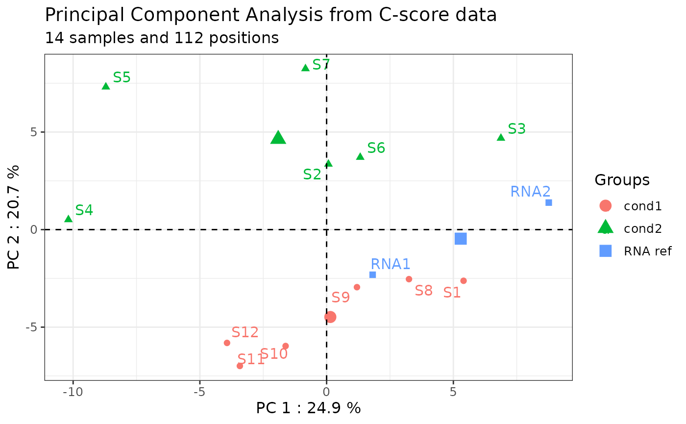

Note: by default, PC1 and PC2 axes are plotted. However, the user can choose the PCA axes of interest using the “axes” argument.

plot_pca(ribo_adjusted,
         color_col = "condition",
         axes = c(2,3), #PC2 and PC3 will be plotted
         only_annotated = TRUE)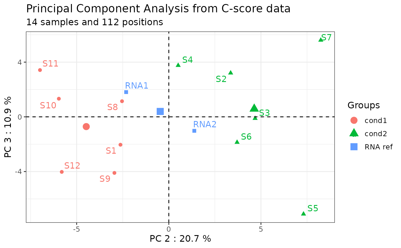

Note: the function returns the complete dudi.pca object (dudi.pca() function from ade4 library) instead of the plot by setting object_only to TRUE:

pca <- plot_pca(ribo_adjusted,
         color_col = "condition",
         only_annotated = TRUE,
         object_only = TRUE)

Comments

A comment section is available in the 2’Ome profiling report to add some personal comments. To do so, a Rmarkdown file should be created and saved in the working directory. Then, path to this report should be given in the comments argument of the report_2ome_site() function.

report_2ome_sites(ribo_adjusted, specie = "human", condition_col = "condition", project_name = "name_of_project", comments =  "./path/to/comments_for_this_report.Rmd")

2’Ome site-by-site report

A site-by-site 2’Ome comparison report can be automatically generated. It uses several metrics and statistical tests to identify differentially 2’Ome sites between biological conditions. To run these functions, a Comparison table and an updated metadata/RiboClass needs to be generated (see Analysis design for multiple comparisons)

report_diff_sites(ribo = ribo_adjusted, specie = "human", condition_col = "comp1", project_name = "name", comparisons = comparisons, comments = "./path/to/comments_for_this_report.Rmd")

To determine whether 2’Ome levels is different between conditions at each site, several functions have been implemented to obtain an html report. Here is a list of the implemented plots/dataframe with the function name:

line plot using the mean C-score of all annotated 2’Ome sites (plot_global_profile())
histogram plot representing differences in the median C-score (plot_comparison_median())
boxplot showing the mean C-scores for each conditions, but only for sites where a statistical difference was observed (ANOVA, Welch, Kruskal-Wallis, Wilcoxon) (plot_stat())
dataframe providing the metrics used to generate the report (get_diff_sites_summary())

Summary table of statistical tests

To get a table of significant sites in at least one test the function below can be used.

get_diff_sites_summary(ribo = ribo_toy, condition_col = "comp1", comparisons = comparisons)

Comments

A comment section is available in the site-by-site 2’Ome comparison report to add some personal comments. To do so, a Rmarkdown file should be created and saved in the working directory. Then, path to this report should be given in the comments argument of the report_diff_sites() function.

report_diff_sites(ribo = ribo_toy, specie = "human", condition_col = "comp1", comparisons = comparisons, comments = "./path/to/comments_for_this_report.Rmd")

Exporting data

Data can be exported as two different objects in three different ways.

Export as a dataframe

The user can export data as a dataframe using the extract_data() function.

By default, C-scores for all the genomic rRNA positions are exported.

ribo_df <- extract_data(ribo_adjusted,
                        col = "cscore")

The user can export data related to the subset of annotated rRNA 2’Ome sites by setting the only_annotated argument to TRUE.

ribo_df <- extract_data(ribo_adjusted,
                        col = "cscore",
                        only_annotated = TRUE)

Excerpt from the output dataframe, where S1, S2 and S3 are samples:
site	S1	S2	S3
18S_Am27	0.9783333	0.9745514	0.9810412
18S_Am99	0.9680204	0.9646470	0.9724150
18S_Um116	0.9276274	0.9470968	0.9407083
18S_Um121	0.9630216	0.9684459	0.9691576
18S_Am159	0.9629730	0.9620986	0.9686766
18S_Am166	0.9809492	0.9744627	0.9744998
18S_Um172	0.9510189	0.9400922	0.9517981
18S_Cm174	0.9119119	0.8668456	0.8806886
18S_Um354	0.9709273	0.9722054	0.9756174
18S_Um428	0.9268668	0.9276018	0.9504224

Export as a ggplot-ready dataframe

The user can export data as a ggplot-ready dataframe using the format_to_plot() function.

By default, C-scores for all the genomic rRNA positions are exported. The user can export additional information contained in the metadata by specifying the name of the column of interest. The user can export information related to the subset of annotated rRNA 2’Ome sites by setting the only_annotated argument to TRUE.

Here is an example of ggplot-ready dataframe containing the C-scores of all the genomic rRNA positions as well as the condition related to the particular sample of interest:

ggplot_table <- format_to_plot(ribo = ribo_adjusted, metadata_col = "condition", only_annotated = FALSE)

Excerpt from the output ggplot-ready dataframe
	sample	site	cscore	condition
501	RNA1	18S_0501	0.0000000	RNA ref
502	RNA1	18S_0502	0.2601804	RNA ref
503	RNA1	18S_0503	0.0000000	RNA ref
504	RNA1	18S_0504	0.3179712	RNA ref
505	RNA1	18S_0505	0.5132894	RNA ref
506	RNA1	18S_0506	0.6354548	RNA ref
507	RNA1	18S_0507	0.0000000	RNA ref
508	RNA1	18S_0508	0.0000000	RNA ref
509	RNA1	18S_0509	0.0000000	RNA ref
510	RNA1	18S_0510	0.9380812	RNA ref

Export as a dataframe by condition

The mean_samples_by_condition() function regroup all the genomic rRNA positions by condition and compute mean and standard deviation for each condition. Then it displays a table.

By default, the function provides the metrics of the C-scores. By setting the value argument to “count”, it is also possible to calculate these values from the read-end counts. Calculations can be limited to only annotated rRNA 2’Ome sites by setting the only_annotated argument to TRUE.

Here is an example of dataframe showing the summarized C-scores per modality of the “condition” variable for all the genomic rRNA positions:

mean_tb <- mean_samples_by_condition(ribo_adjusted,
                                    value = "cscore", #or "count"
                                    metadata_condition = "condition",
                                    only_annotated = TRUE)

Excerpt from the output dataframe by condition
site	condition	mean	sd
18S_Am1031	RNA ref	0.9749922	0.0047461
18S_Am1031	cond1	0.9703699	0.0032725
18S_Am1031	cond2	0.9723714	0.0057723
18S_Am1383	RNA ref	0.9796876	0.0035939
18S_Am1383	cond1	0.9765212	0.0027083
18S_Am1383	cond2	0.9779684	0.0028759
18S_Am159	RNA ref	0.9684126	0.0022025
18S_Am159	cond1	0.9609920	0.0054882
18S_Am159	cond2	0.9623362	0.0065239
18S_Am166	RNA ref	0.9826490	0.0033169

Session info

sessionInfo()
#> R version 4.5.1 (2025-06-13)
#> Platform: x86_64-pc-linux-gnu
#> Running under: Ubuntu 24.04.3 LTS
#> 
#> Matrix products: default
#> BLAS:   /usr/lib/x86_64-linux-gnu/openblas-pthread/libblas.so.3 
#> LAPACK: /usr/lib/x86_64-linux-gnu/openblas-pthread/libopenblasp-r0.3.26.so;  LAPACK version 3.12.0
#> 
#> locale:
#>  [1] LC_CTYPE=C.UTF-8       LC_NUMERIC=C           LC_TIME=C.UTF-8       
#>  [4] LC_COLLATE=C.UTF-8     LC_MONETARY=C.UTF-8    LC_MESSAGES=C.UTF-8   
#>  [7] LC_PAPER=C.UTF-8       LC_NAME=C              LC_ADDRESS=C          
#> [10] LC_TELEPHONE=C         LC_MEASUREMENT=C.UTF-8 LC_IDENTIFICATION=C   
#> 
#> time zone: UTC
#> tzcode source: system (glibc)
#> 
#> attached base packages:
#> [1] stats     graphics  grDevices utils     datasets  methods   base     
#> 
#> other attached packages:
#> [1] rRMSAnalyzer_3.0.0 kableExtra_1.4.0   DT_0.34.0          dplyr_1.1.4       
#> 
#> loaded via a namespace (and not attached):
#>   [1] colorRamp2_0.1.0        DBI_1.2.3               rlang_1.1.6            
#>   [4] magrittr_2.0.3          clue_0.3-66             GetoptLong_1.0.5       
#>   [7] ade4_1.7-23             matrixStats_1.5.0       compiler_4.5.1         
#>  [10] RSQLite_2.4.3           mgcv_1.9-3              png_0.1-8              
#>  [13] systemfonts_1.2.3       vctrs_0.6.5             sva_3.56.0             
#>  [16] stringr_1.5.2           pkgconfig_2.0.3         shape_1.4.6.1          
#>  [19] crayon_1.5.3            fastmap_1.2.0           XVector_0.48.0         
#>  [22] backports_1.5.0         labeling_0.4.3          rmarkdown_2.29         
#>  [25] UCSC.utils_1.4.0        ragg_1.5.0              purrr_1.1.0            
#>  [28] bit_4.6.0               xfun_0.53               cachem_1.1.0           
#>  [31] GenomeInfoDb_1.44.2     jsonlite_2.0.0          blob_1.2.4             
#>  [34] BiocParallel_1.42.1     broom_1.0.9             parallel_4.5.1         
#>  [37] cluster_2.1.8.1         R6_2.6.1                bslib_0.9.0            
#>  [40] stringi_1.8.7           RColorBrewer_1.1-3      limma_3.64.3           
#>  [43] genefilter_1.90.0       car_3.1-3               jquerylib_0.1.4        
#>  [46] Rcpp_1.1.0              iterators_1.0.14        knitr_1.50             
#>  [49] IRanges_2.42.0          Matrix_1.7-3            splines_4.5.1          
#>  [52] tidyselect_1.2.1        rstudioapi_0.17.1       abind_1.4-8            
#>  [55] yaml_2.3.10             doParallel_1.0.17       codetools_0.2-20       
#>  [58] lattice_0.22-7          tibble_3.3.0            KEGGREST_1.48.1        
#>  [61] Biobase_2.68.0          withr_3.0.2             S7_0.2.0               
#>  [64] evaluate_1.0.5          survival_3.8-3          desc_1.4.3             
#>  [67] xml2_1.4.0              Biostrings_2.76.0       circlize_0.4.16        
#>  [70] pillar_1.11.0           ggpubr_0.6.1            MatrixGenerics_1.20.0  
#>  [73] carData_3.0-5           foreach_1.5.2           stats4_4.5.1           
#>  [76] generics_0.1.4          S4Vectors_0.46.0        ggplot2_4.0.0          
#>  [79] scales_1.4.0            xtable_1.8-4            glue_1.8.0             
#>  [82] tools_4.5.1             locfit_1.5-9.12         annotate_1.86.1        
#>  [85] ggsignif_0.6.4          fs_1.6.6                XML_3.99-0.19          
#>  [88] grid_4.5.1              tidyr_1.3.1             edgeR_4.6.3            
#>  [91] AnnotationDbi_1.70.0    colorspace_2.1-1        nlme_3.1-168           
#>  [94] GenomeInfoDbData_1.2.14 Formula_1.2-5           cli_3.6.5              
#>  [97] textshaping_1.0.3       viridisLite_0.4.2       svglite_2.2.1          
#> [100] ComplexHeatmap_2.24.1   gtable_0.3.6            rstatix_0.7.2          
#> [103] sass_0.4.10             digest_0.6.37           BiocGenerics_0.54.0    
#> [106] ggrepel_0.9.6           rjson_0.2.23            htmlwidgets_1.6.4      
#> [109] farver_2.1.2            memoise_2.0.1           htmltools_0.5.8.1      
#> [112] pkgdown_2.1.3           factoextra_1.0.7        lifecycle_1.0.4        
#> [115] httr_1.4.7              statmod_1.5.0           GlobalOptions_0.1.2    
#> [118] bit64_4.6.0-1           MASS_7.3-65

References

Birkedal, Ulf, Mikkel Christensen-Dalsgaard, Nicolai Krogh, Radhakrishnan Sabarinathan, Jan Gorodkin, and Henrik Nielsen. 2014. “Profiling of Ribose Methylations in RNA by High-Throughput Sequencing.” Angewandte Chemie International Edition, November, n/a–. https://doi.org/10.1002/anie.201408362.

Erales, Jenny, Virginie Marchand, Baptiste Panthu, Sandra Gillot, Stéphane Belin, Sandra E. Ghayad, Maxime Garcia, et al. 2017. “Evidence for rRNA 2′-o-Methylation Plasticity: Control of Intrinsic Translational Capabilities of Human Ribosomes.” Proceedings of the National Academy of Sciences 114 (49): 12934–39. https://doi.org/10.1073/pnas.1707674114.

Marcel, Virginie, Janice Kielbassa, Virginie Marchand, Kundhavai S Natchiar, Hermes Paraqindes, Flora Nguyen Van Long, Lilia Ayadi, et al. 2021. “Ribosomal RNA 2’ O-methylation as a novel layer of inter-tumour heterogeneity in breast cancer.” NAR Cancer 3 (1). https://doi.org/10.1093/narcan/zcab006.

Marchand, Virginie, Florence Blanloeil-Oillo, Mark Helm, and Yuri Motorin. 2016. “Illumina-based RiboMethSeq approach for mapping of 2’-O-Me residues in RNA.” Nucleic Acids Research 44 (16): e135–35. https://doi.org/10.1093/nar/gkw547.

Théo COMBE, Hermès PARAQINDES, Allyson MOUREAUX, Janice KIELBASSA, Fleur BOURDELAIS, Sébastien DURAND, Emilie THOMAS, Anthony FERRARI and Virginie MARCEL

09/12/2025

General information

Help, bug reports and suggestions

Acknowledgements

Funding

Installation

Initial preparation of the dataset

RiboClass

Loading data

Data to provide

Read-end counts

Metadata

How to load the data

rRNA names

Provided

Custom

C-score calculation

What is a C-score ?

C-score computation when loading data

C-score computation during the analysis

Quality control

Content of the QC report

Correlation matrix

Output of the QC report

Comments

Batch effect

Batch effect identification

Batch effect adjustment

Verifying local coverage

Data formatting for subsequent analyses

Sample manipulation

Keep or remove samples

rRNA manipulation and annotation

rRNA manipulation

Remove rRNA

Rename rRNA

Annotation of rRNA 2’Ome sites

Included annotation : Human 2’Ome rRNA sites

Customize 2’Ome sites annotations

Annotate rRNA sites

Analysis design for multiple comparisons

Addition of new columns in the metadata

(i) Update of the metadata .csv file

(ii) create a new Riboclass:

Comparison table

(i) Creation of the dataframe for the report_diff_sites function:

(ii) Creation of a new RiboClass including only the required samples

2’Ome profiling report

PCA

Comments

2’Ome site-by-site report

Summary table of statistical tests

Comments

Exporting data

Export as a dataframe

Export as a ggplot-ready dataframe

Export as a dataframe by condition

Session info

References